Differential Equations Formula Cheat Sheet and Methods

Differential equations formula cheat sheet provides important methods, solutions, and formulas to solve equations involving rates of change, widely used in physics, engineering, and real-world modelling. Mathematical equations that include derivatives and which describe the change of quantities with time are known as differential equations. They find extensive application in physics, engineering, biology and economics. Differential equations are used to model real-life systems, including population growth, motion and heat transfer. Differential equations can be in various forms, such as ordinary and partial differential equations. The solution of these equations enables us to understand and predict how systems behave. They play a critical role in the study of natural phenomena as well as in engineering processes.

Differential Equations Formula Cheat Sheet

Topic	Formula	Description
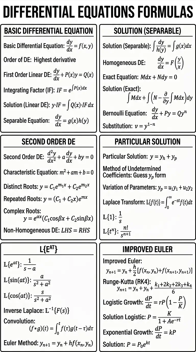
Basic Differential Equation	dy/dx = f(x, y)	General form
Order of DE	Highest derivative	Degree of equation
First Order Linear DE	dy/dx + P(x)y = Q(x)	Standard form
Integrating Factor (IF)	IF = e^(∫P(x)dx)	Solve linear DE
Solution (Linear DE)	y·IF = ∫Q(x)·IF dx	General solution
Separable Equation	dy/dx = g(x)h(y)	Separate variables
Solution (Separable)	∫dy/h(y) = ∫g(x)dx	Integrate both sides
Homogeneous DE	dy/dx = F(y/x)	Substitution y = vx
Exact Equation	Mdx + Ndy = 0	Exact if dM/dy = dN/dx
Solution (Exact)	∫Mdx + ∫(N − ∂/∂y ∫Mdx)dy	Solve exact DE
Bernoulli Equation	dy/dx + Py = Qyⁿ	Nonlinear DE
Substitution	v = y^(1−n)	Convert to linear
Second Order DE	d²y/dx² + a dy/dx + by = 0	General form
Characteristic Equation	m² + am + b = 0	Solve roots
Distinct Roots	y = C₁e^(m₁x) + C₂e^(m₂x)	General solution
Repeated Roots	y = (C₁ + C₂x)e^(mx)	Solution form
Complex Roots	y = e^(αx)(C₁cosβx + C₂sinβx)	Oscillatory solution
Non-Homogeneous DE	LHS = RHS	Particular solution needed
Particular Solution	y = yₕ + yₚ	Complete solution
Method of Undetermined Coefficients	Guess yₚ form	Solve RHS type
Variation of Parameters	yₚ = u₁y₁ + u₂y₂	General method
Laplace Transform	L{f(t)} = ∫₀^∞ e^(-st)f(t)dt	Transform method
L{1}	1/s	Basic transform
L{tⁿ}	n!/sⁿ⁺¹	Power function
L{e^(at)}	1/(s−a)	Exponential
L{sin(at)}	a/(s² + a²)	Trig transform
L{cos(at)}	s/(s² + a²)	Trig transform
Inverse Laplace	L⁻¹{F(s)}	Back to time domain
Convolution	(f*g)(t) = ∫₀ᵗ f(τ)g(t−τ)dτ	Integral relation
Euler Method	yₙ₊₁ = yₙ + h f(xₙ,yₙ)	Numerical method
Improved Euler	yₙ₊₁ = yₙ + h/2 [f(xₙ,yₙ)+f(xₙ₊₁,yₙ₊₁)]	Better approx
Runge-Kutta (RK4)	yₙ₊₁ = yₙ + (k₁+2k₂+2k₃+k₄)/6	High accuracy
Logistic Growth	dP/dt = rP(1 − P/K)	Population model
Solution Logistic	P = K / (1 + Ae^(−rt))	Growth formula
Exponential Growth	dP/dt = kP	Growth model
Solution	P = P₀e^(kt)	Exponential solution

Download PDF

Conclusion Differentiation equations enhance analytical skills and problem-solving. It is based on calculus and algebra. Differential equations are applied by engineers to design or analyse performance. They are applied by scientists in the study of physical laws and natural processes. Computer simulations and modeling also involve the use of differential equations. Knowing these equations will assist in solving complicated problems in real life. In general, differential equations form an important aspect of advanced mathematics and have extensive applications. In conclusion, differential equations are important for modeling real-world changes and systems. They are widely used in science and engineering to solve complex problems.